保序回归-IsotonicRegression
1. 保序回归的数学定义
定义:给定一个有限的实数集合 $Y=y_1, y_2, \cdots, y_n$ 代表观察到的响应,以及 $X = x_1, x_2, \cdots, x_n$ 代表未知的响应值,训练一个模型最小化下列方程:
其中 $x_1 \le x_2 \cdots \le x_n$, $w_i$ 为权重是正值,其结果称之为保序回归,而且其解是唯一的。
保序回归的结果是分段函数。
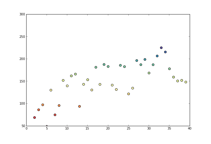
2. 举例说明
一般从元素的首元素向后观察,如果出现乱序现象 (当前元素大于后续元素) 时停止观察,并从乱序元素开始逐个向前吸收元素组成一个序列,直达该序列所有元素的平均值小于或是等于下一个待吸收的元素。
未发现乱序正常读取
1
2
原始序列:<9, 10, 14>
结果序列:<9, 10, 14>分析:从9往后观察,到最后的元素14都未发现乱序情况,不用处理。
发现乱序,平均值大于后面小于前面
1
2
原始序列:<9, 14, 10>
结果序列:<9, 12, 12>分析:从9往后观察,观察到14时发生乱序 (14 > 10),停止该轮观察,转入吸收元素处理,从吸收元素10向前一个元素的子序列为 <14, 10>,取该序列所有元素的平均值得12,故用序列 <12, 12> 替代 <14, 10>。吸收10后已经到了最后的元素,处理操作完成。
发现乱序,平均值大于后面,大于前面
1
2
原始序列:<14, 9, 10, 15>
结果序列:<11, 11, 11, 15>分析:从14往后观察时发生乱序 (14 > 9),停止该轮观察转入吸收元素处理,吸收元素9后子序列为 <14, 9>。求该序列所有元素的平均值得11.5,由于11.5大于下个待吸收的元素10,所以再吸收10得序列 <14, 10 9,>。求该序列所有元素的平均值得11,由于11小于下个待吸收的元素15,所以停止吸收操作,用序列 <11, 11 11,> 替代 <14, 10 9,>。
3. 官方代码
1 | # Author: Nelle Varoquaux <nelle.varoquaux@gmail.com> |
输出结果:
1 | index before after |
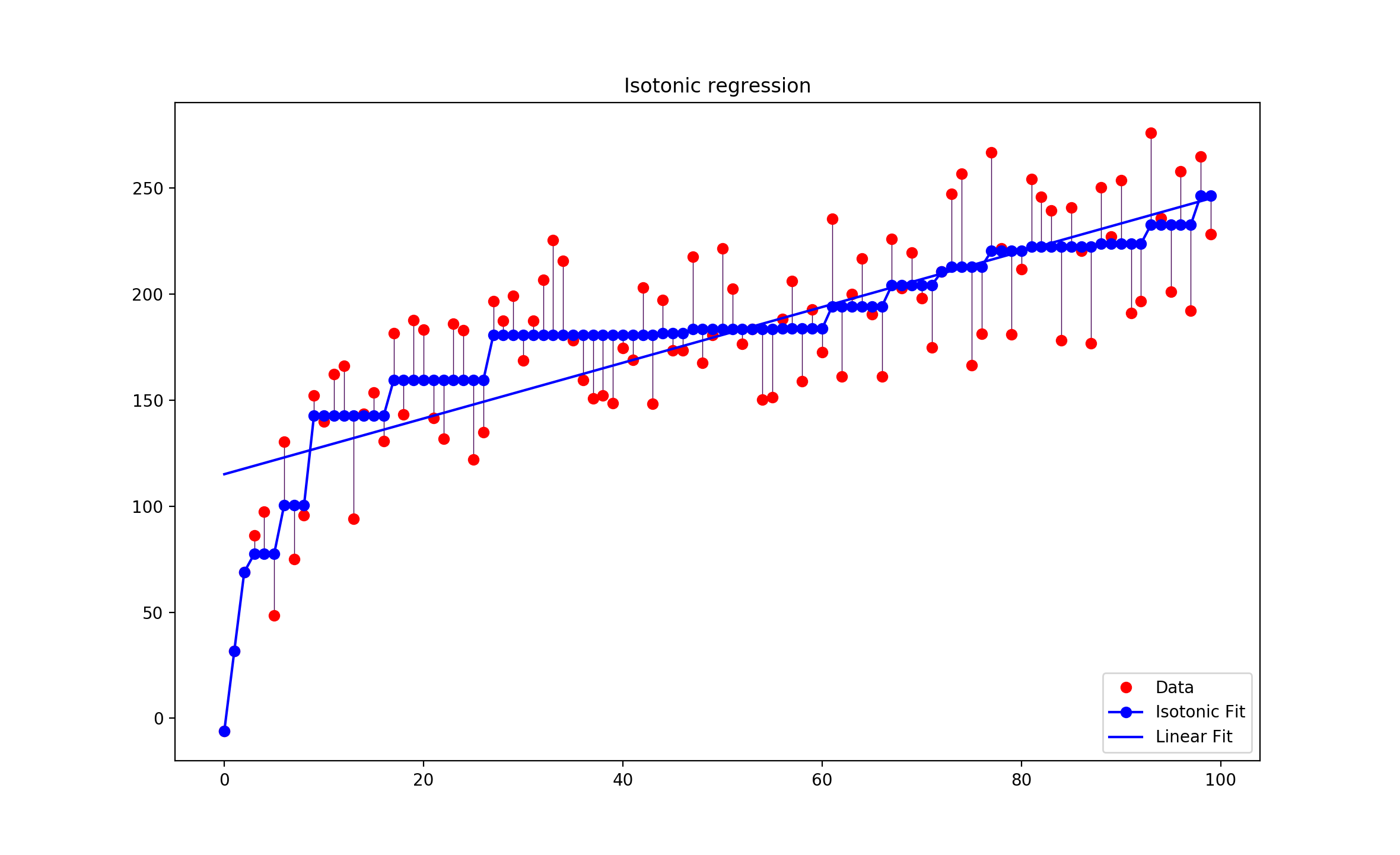
4. 保序回归应用实例
以某种药物的使用量为例,假设药物使用量为数组 $X=0, 1, 2, 3, \cdots, 99$,病人对药物的反应量为$Y = y_1, y_2, y_3, \cdots, y_{99}$ ,而由于个体的原因,$Y$不是一个单调函数(即:存在波动),如果我们按照药物反应排序,对应的$X$就会成为乱序,失去了研究的意义。而我们的研究的目的是为了观察随着药物使用量的递增,病人的平均反应状况。在这种情况下,使用保序回归,即不改变$X$的排列顺序,又求的$Y$的平均值状况。
从上图中可以看出,最长的蓝线 $x$ 的取值约是$30$到$60$,在这个区间内,$Y$的平均值一样,那么从经济及病人抗药性等因素考虑,使用药量为30个单位是最理想的。
当前IT行业虚拟化比较流行,使用这种方式,找到合适的判断参数,就可以使用此算法使资源得到最大程度的合理利用。